![]()
Supervised by Prof. Gianluca Moro,
Dr. Giacomo Frisoni and Dr. Lorenzo Molfetta
2025-07-24
Problem
- Context ⚽
- Over recent years, sports data analysis has gone from basic post game stats to using detailed time and space information to shape tactics, evaluate players and guide decisions during matches.
- Our Task: Shot Prediction
- Objective: Identify soccer actions that are likely to lead to a shot and quantify each player’s contribution to those actions.
- Our Method:
- Develop a Graph Neural Network that, as an oracle, ingests the current game state (capturing evolving spatio-temporal patterns) and outputs the probability of a shot.
- On top of that we want to understand the network’s probability outputs to uncover the patterns and features that drive its predictions.
Machine Learning on Graphs
Why graphs?
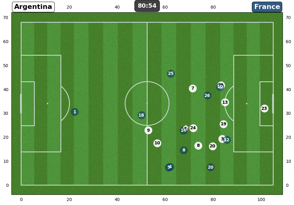
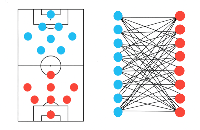
- Graphs effectively represent spatial interactions between players, capturing and modelling the complexity of soccer.
- Node features embed informations about each player.
- Edge connections define how relationships between players are represented and influence message flow in the network.
- Node features embed informations about each player.
- We model the problem as a complete weighted bipartite graph where each player is connected to every opponent.
- Inspired by Google DeepMind TacticAI and Goka et al.
- Graphs effectively represent spatial interactions between players, capturing and modelling the complexity of soccer.
Why bipartite connection?
This type of connection can reflect both direct proximity to opponents and the local defensive/offensive support structure.
When extended to a two-hop view, this construction captures:
- 1-hop edges → how many opposing players are nearby.
- 2-hop edges → how many of a player’s own teammates are near those opponents.
Why weight the edges?
- Nearby interactions matter most, so we apply an exponential decay to pairwise distances, down weighting distant players and highlighting close ones.
- Thus, edge weights are computed as \(w_{ij} = e^{-d_{ij}}\), where \(d_{ij} = \lVert {p}_i - {p}_j\rVert_2\) and \({p}_i, {p}_j\) denote the 2D field coordinates of players \(i\) and \(j\).
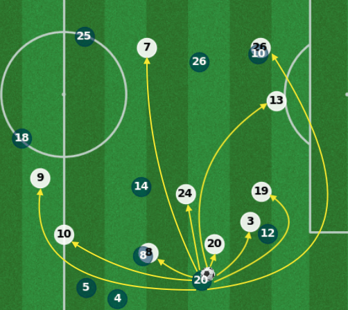 No weights
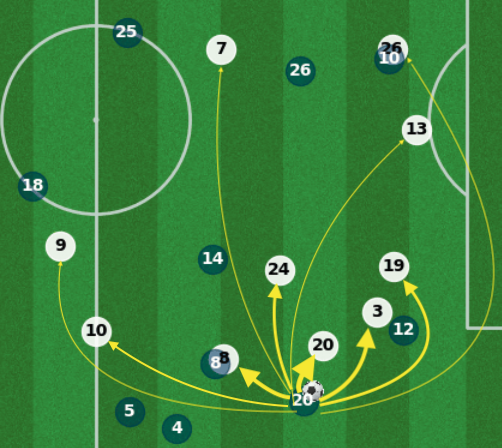 With weights
Dataset
Data Sources & Statistics
- Dataset: FIFA World Cup 2022 (PFF.com)
- 64 matches total:
- 48 group-stage → training set
- 16 knockout → validation set
- Tracking Data: camera-based, frame-by-frame positions (30 fps)
- Event Data: manually labeled actions (passes, shots, etc.)
- Additional Player Statistics: player profiles and performance scraped from TransferMarkt & FBRef
- 64 matches total:
- Focus: Event Data
- We enrich each event computing every player’s speed and direction with the 60 preceding tracking frames.
- In total we analyze 19 048 frames, organised into chains that capture individual football actions.
- Chain Statistics:
- 3 716 total chains
- 2 546 Negative chains
- 1 170 Positive chains
- 2 546 Negative chains
- 3 716 total chains
![]()
![]()
![]()
Feature Engineering & Normalization
- Spatial features
- x, y → player position scaled by pitch dimensions ([0,1])
- vx,vy → velocity components
- sinθ, cosθ → player’s direction ([-1,1])
- ball_dist → distance between player and ball ([0,1])
- ball_direction_sim → cosine similarity between player and ball direction ([-1,1])
- dz → distance between player and ball’s z-axis coordinate ([0,1])
- Categorical (one-hot):
- is_ball_carrier → the player has possession of the ball
- is_possession_team → the player’s team has the ball
- player_Role → player’s tactical role
- Global features:
- possesionEventType: type of possession action (one-hot)
- frameTime: timestamp of the current frame (z-score)
- duration: length of the possession event in seconds (z-score)
- Player Stats
- Player Metadata → height, weight, market value (z-score)
- Player Shooting stats → goals, shots, etc. (z-score)
Method
- Workflow: From Frames to Chains
- First attempt: We treated each frame as an independent sample and trained the network on these single frames, as they constituted a very large pool of training examples.
- Problem: After several unsuccessful experiments, we realised that ignoring temporal dynamics severely limited the model’s performance on this task.
- Solution: We encoded football actions as sequences of graphs of arbitrary length during which one team maintains possession of the ball.
- Augmentation: We achieved a 4× increase in the dataset by mirroring each sequence across the pitch, giving us a much larger pool of training examples.
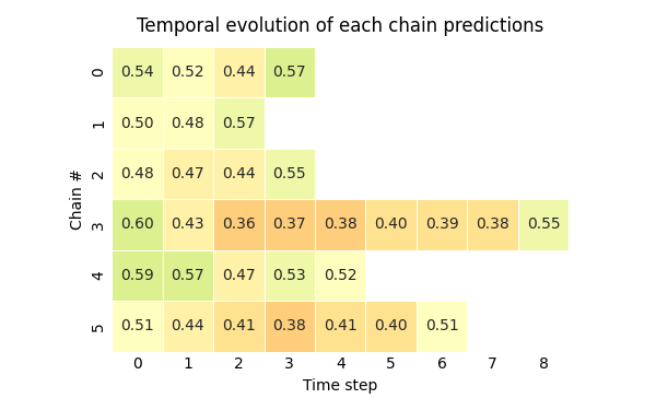
- Temporal approach (Many-to-Many)
- Input: A sequence of graphs \(\mathbf{G_1, G_2, \dots, G_T}\), one for each timestep \(\mathbf{t} \in \{1, \dots, T\}\).
- Architecture:
- A backbone to extract spatial informations from the input graph
- A neck to readout and for temporal processing
- An head (MLP with dropout) for prediction
- Output: For every timestep \(\mathbf{t}\), a probability \(\mathbf{{p}_t}\) that the current possession state will result in a shot.
![]()
![]()

Architecture: Backbones
- Baselines
- Advanced:
GCNII → deep GCN with initial residual + identity mapping to enable deep networks and extract deep features. 🔗
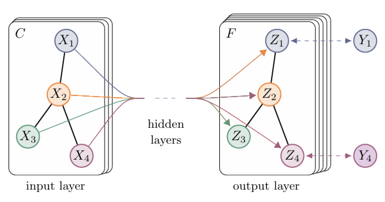
GATv2 → dynamic attention assigns importance weights to edges enabling adaptive weighted message passing to scale down less important nodes and emphasize more important ones. 🔗
GINE → it matches the power of the 1-WL which can distinguish most graph classes by implementing the aggregation step as an injective function approximating it with a MLP, making it an exceptionally expressive GNN. GIN 🔗 - GINE 🔗
- Other approches:
- GPS → a hybrid architecture that combines MPNN with graph transformers, reaching expressiveness beyond 1-WL and achieving SOTA results. 🔗
- GNN+ → every message-passing is encapsulated in a wrapper with normalization, dropout, skip connection and a FFN, producing an architecture matching the performance of Graph Transformer. 🔗
- Diffpool → uses differentiable hierarchical pooling to build coarser representations of graphs before the final readout. 🔗
 Kipf et al. Graph Convolutional Network
 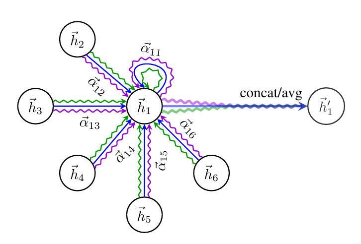 Velicković et al. GAT attention
 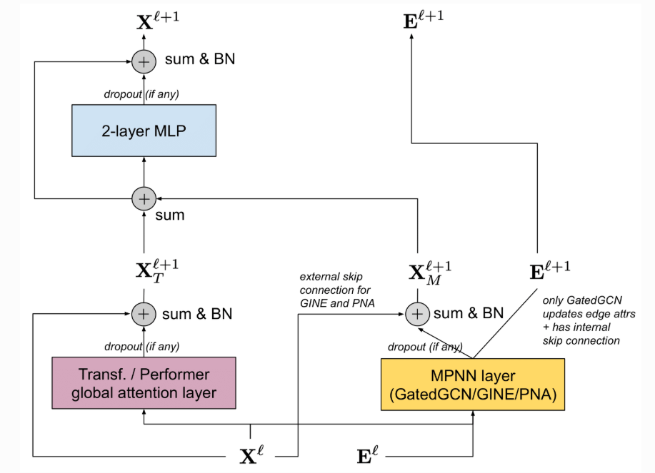 Rampášek et al. GPS Layer
Architecture: Necks
- Readout
- A pooling operation is applied to the backbone’s output to obtain a graph embedding.
- Fusion
- A projection layer takes the global features as input and produces a global embedding.
- The graph and global embeddings are then concatenated into a fused embedding.
- Two main modalities:
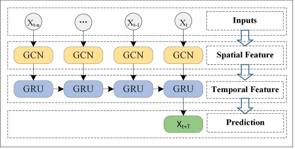
- Graph → Following the T-GCN architecture, the output embeddings from the backbone are passed through first a readout layer, then a fusion module and lastly a RNN cell to compute the next hidden state. Final predictions are based only on these hidden states, clearly separating spatial feature extraction from temporal modeling.
- Node → Both the backbone and the GCRN process spatio-temporal information at each timestep. However, only the output of the backbone is passed through a readout layer, followed by a fusion module and a prediction head to produce the final output.
- RNN type
- GRU/LSTM for graph mode
- GConvGRU/GConvLSTM for node mode
 Zhao et al. T-GCN architecture
 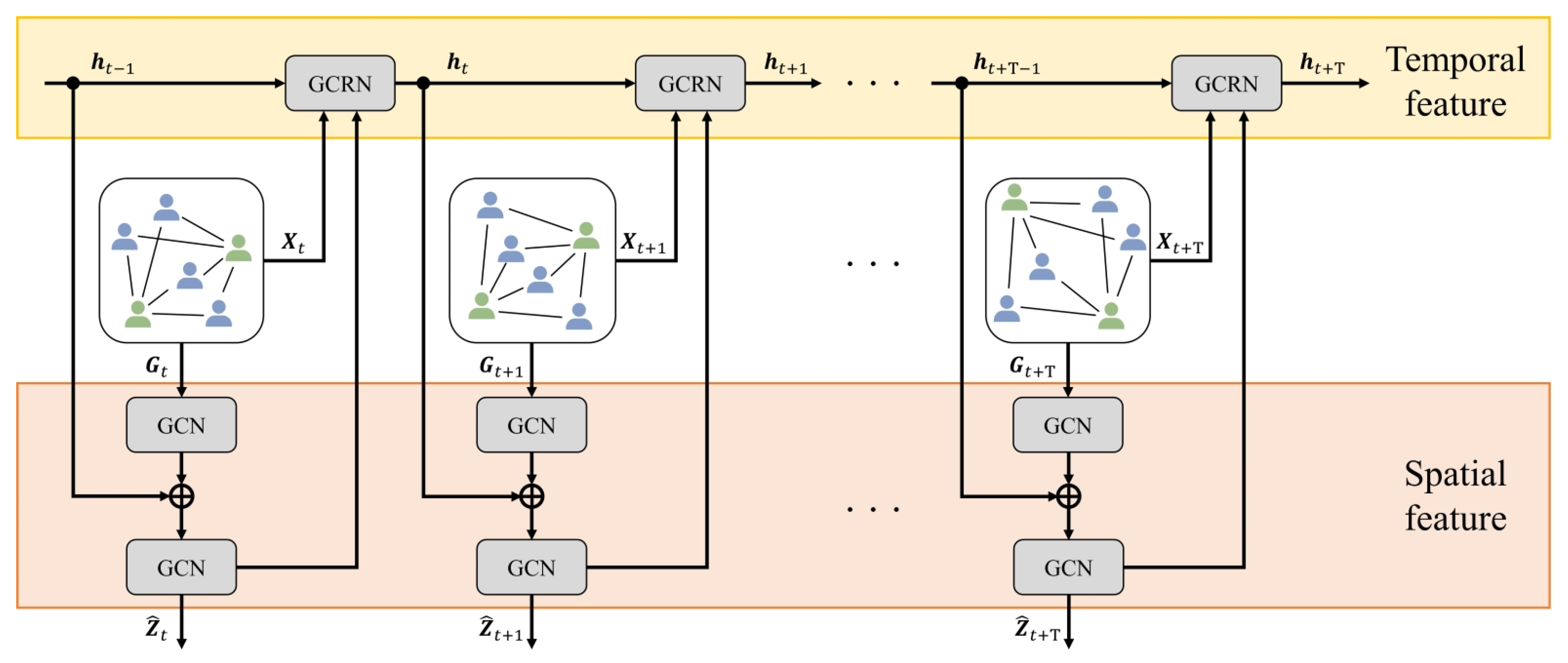 Goka et al. GCRN architecture
Explainability
GNN Explainer
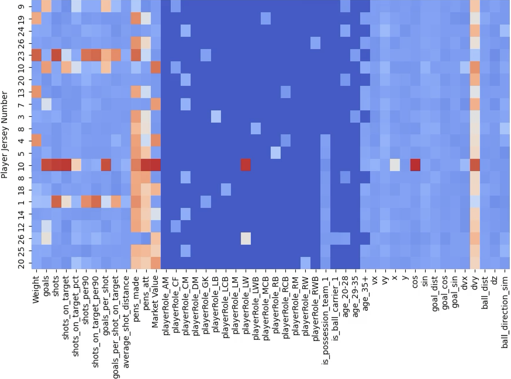
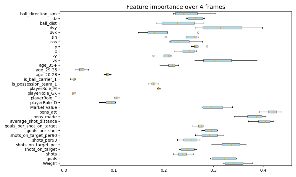
- GNNExplainer identifies a compact subgraph and a small subset of node features critical to the GNN’s prediction. 🔗
- By visualizing the learned masks below, we can highlight the key player interactions and feature contributions that drive each prediction.